Raccoon Image Classifier

App

Introduction

So, fun fact about me, I have never deployed a Neural Network (NN) before.

There’s never been a need to in my line of work, nor in my hobby data projects. The data I work with is overwhelmingly in tabular format, thus tree-based methods or linear models are almost always preferred. They’re ‘simpler’, faster, and the performance differences are negligible to the point at which I don’t bother to learn one of Tensorflow or Pytorch. Further, I really don’t enjoy fitting something I don’t understand, and NNs are very complicated. Despite still not understanding the finer details of NNs, I’ve finally fit one… to classify pictures of raccoons.

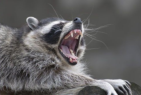
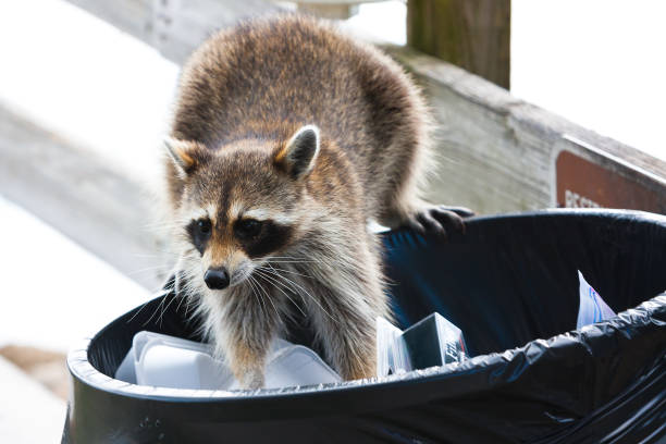
Why raccoons? Because they’re cool little fellas and my favorite animal, as you can probably ascertain from the theming on this website.

The Code

Before getting started, please shove this at the top of your script/notebook and ensure you have these packages installed:

import os # This import was my doing
import PIL
import tensorflow as tf
import pathlib

from tensorflow import keras
from tensorflow.keras import layers
from tensorflow.keras.models import Sequential
from tensorflow.keras import layers, models
from tensorflow.keras.preprocessing.image import ImageDataGenerator

Anyway, this process is a near copy-paste walkthrough from Tensorflow’s image classification tutorial found here. The only things which I altered were the training and testing data to accommodate my goal of classifying raccoons rather than flowers. I would argue that the data procurement step is the most tedious/challenging part of this exercise. Fortunately, once data is secured, the process for ingestion is quite straightforward thanks to keras. We’ll want to set up folders somewhere on our computer containing the images for training, with each folder being named to the class of images contained inside. For example, my folder looked like this:

images/
...raccoon/
......raccoon_1.jpg
......raccoon_2.jpg
...dog/
......dog_1.jpg
......dog2_2.jpg
.
.
.
...something_else/
......human_1.jpg
......tiger_1.jpg
......car_1.jpg

Thankfully, keras can magically take this directory and split them into train/test sets for us by using the following code:

# Will resize images in train/test data to 180x180:
img_height = 180
img_width = 180

# Training set:
train_ds = tf.keras.utils.image_dataset_from_directory(
  data_dir,
  validation_split=0.2,
  subset="training",
  seed=123,
  image_size=(img_height, img_width)
  )

# Testing set:
val_ds = tf.keras.utils.image_dataset_from_directory(
  data_dir,
  validation_split=0.2,
  subset="validation",
  seed=123,
  image_size=(img_height, img_width)
  )

Here, dir_name will be your path to the images folder from the text example. You may set that directory using:

data_dir = pathlib.Path(os.getcwd() + '//images').with_suffix('')

If you want to ensure that the code did its job properly and identified the appropriate folders, you may print the class names the model will be trained for:

# Print to user what the class names are:
class_names = train_ds.class_names
num_classes = len(class_names)
for name in class_names:
    print(f"Class identified: {name}")

Class identified: cat
Class identified: dog
Class identified: possum
Class identified: raccoon
Class identified: something else

The next thing is telling tensorflow/keras how we want the ingestion process to be handled. If we use the AUTOTUNE method on tf.data, it will instruct the program to dynamically pull the data in preparation for training while the model is already running prior data fetches. This will speed the overall training process up.

# TF Autotuner:
AUTOTUNE = tf.data.AUTOTUNE

# More options which cache data in memory for speed and add overfitting precautions.
train_ds = train_ds.cache().shuffle(1000).prefetch(buffer_size=AUTOTUNE)
val_ds = val_ds.cache().prefetch(buffer_size=AUTOTUNE)

Next we can actually write our model by specifying the layers of our Convolutional Neural Network

# Set model layers and overfitting precautions:
model = Sequential([
  layers.RandomFlip("horizontal", input_shape=(img_height, img_width, 3)),
  layers.RandomRotation(0.1),
  layers.RandomZoom(0.1),
  layers.Rescaling(1./255, input_shape=(img_height, img_width, 3)),
  layers.Conv2D(16, 3, padding='same', activation='relu'),
  layers.MaxPooling2D(),
  layers.Conv2D(32, 3, padding='same', activation='relu'),
  layers.MaxPooling2D(),
  layers.Conv2D(64, 3, padding='same', activation='relu'),
  layers.MaxPooling2D(),
  layers.Dropout(0.2),
  layers.Flatten(),
  layers.Dense(128, activation='relu'),
  layers.Dense(num_classes)
])

So, things to go over here: what are each of the methos being called doing?

• RandomFlip does exactly what it sounds like, it’s randomly flipping our images horizontally. This is a measure to help prevent overfitting.
• RandomRotation same logic as above, but with a rotation transformation.
• RandomZoom… you get the idea.
• Rescaling normalizes the data by dividing by the maximum value that a color channel’s ‘intensity’, or brightness takes on.
• Conv2D: This sets the number of neurons/nodes in your NN’s convolutional layers. The number of neurons are determined by the number of filters you place onto the image (in the first call of this method, 16). Filters are effectively windows capturing a portion of your image, set to a given kernal size (in this case, a 3x3 matrix, or ‘window’) which convolutes across your image to create a feature map.
• MaxPooling: This downsamples the spatial dimension of the feature map by selecting the maximum value within your kernel window.
• Dropout: Will randomly drop input data from training to prevent overfitting.
• Flatten: Flattens the input data into a one-dimensional array.
• Dense: This is the dense layer of neurons that take the image processing outputs of prior steps to spit out a final prediction.

Next, we want to set the metric we wish to optimize and which loss function we wish to minimize:

# Configure model:
model.compile(optimizer='adam',
              loss=tf.keras.losses.SparseCategoricalCrossentropy(from_logits=True),
              metrics=['accuracy'])

Now we’re finally able to fit and save our model!

# Fit NN:
epochs=15
history = model.fit(
  train_ds,
  validation_data=val_ds,
  epochs=epochs
)

# Save the model as a TFLite file:
# Convert the model.
converter = tf.lite.TFLiteConverter.from_keras_model(model)
tflite_model = converter.convert()

# Save the model.
with open('raccoon.tflite', 'wb') as f:
  f.write(tflite_model)

Results.

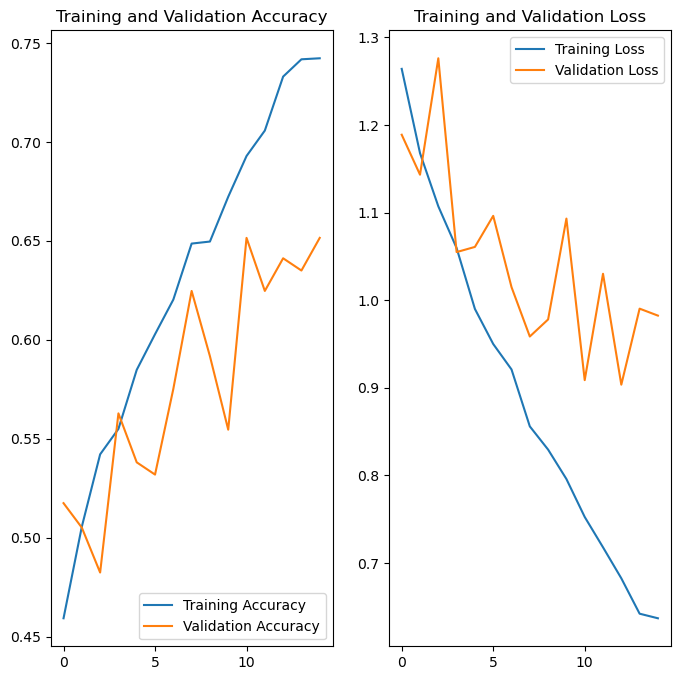
After running the NN through 15 epochs, we’ve achieve about a 60% test set accuracy marginally. However, it would seem that the model has learned to over-rely on classifying unkown images as dogs. This is likely due to the quality and sample dize differences between the pictures of dogs I had, and the pictures of everything else. One potential solution would be to blur images prior to training, which will be investigated on the next post!

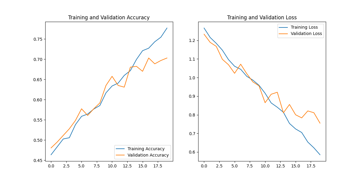
UPDATE

I’ve added Gaussian blurring to the images, and it looks like we’re getting a bit more accuracy now! Below is a custom layer class that will apply the blur for us:

import tensorflow as tf
from tensorflow.keras import layers

class GaussianBlur(layers.Layer):
    def __init__(self, filter_size=3, sigma=1., **kwargs):
        super().__init__(**kwargs)
        self.filter_size = filter_size
        self.sigma = sigma

    def build(self, input_shape):
        # Create a 2D Gaussian filter.
        x = tf.range(-self.filter_size // 2, self.filter_size // 2 + 1, dtype=tf.float32)
        x = tf.exp(-0.5 * (x / self.sigma) ** 2)
        x /= tf.reduce_sum(x)
        gaussian_filter = tf.tensordot(x, x, axes=0)
        gaussian_filter = tf.reshape(gaussian_filter, (*gaussian_filter.shape, 1, 1))
        n_channels = input_shape[-1]
        self.gaussian_filter = tf.repeat(gaussian_filter, n_channels, axis=-2)

    def call(self, inputs):
        return tf.nn.depthwise_conv2d(inputs, self.gaussian_filter, strides=[1, 1, 1, 1], padding='SAME')

I also updated the model to pass through 20 epochs instead of 15. The plots showing the train/test accuracy and loss at each epoch is shown below:

Resources/References:

• Tensorflow Image Classifier tutorial: https://www.tensorflow.org/tutorials/images/classification
• Helpful Medium Article for intuition: https://towardsdatascience.com/each-convolution-kernel-is-a-classifier-5c2da17ccf6e