Survival Analysis Simulation
Intro
Hey there! This is an old post dating back to 2022, but this will serve as my first blog-post on my newest website (the one you’re on). I plan on keeping the majortity of my posts sports & stats centric, but from time to time I may plop in something like this. Plus, it’s super useful for me to look back on this sort of stuff whenever it comes up in my professional work.
Anyway, the content below is a Survival Analysis censoring simulation that I worked on while in graduate school.
Problem
Discover how censored data impacts estimation bias:
The task is outlined as follows:
- Let event time be defined by $X\space \sim \space Exp(\lambda)$ and censoring time $Y\space \sim \space Exp(\mu)$.
We have two types of data:
Right censoring data, generated by $Z_i\space = \space min(X_i, Y_i)$ and $\Delta_i\space=\space 1[X_i\le Y_i]$ for $i = 1,2,…,n$
Current status, interval censored data generated by $Z_i\space = \space Y_i$ and $\Delta_i\space=\space 1[X_i\le Y_i]$ for $i = 1,2,…,n$
Use this informtion in tandem with the below instructions to observe estimation bias for different types and levels of censoring.
Instructions:
(Monte-Carlo simulation experiment):
Consider a Monte-Carlo simulation study to compare the two MLEs under the following setting:
• Choose the true parameter $\lambda$ = 5
• Choose the parameter $\mu$ according to the censoring rate $CP=Pr(X > Y)$
• Generate $n$ independent paired observations $(x_i; y_i), \space i = 1, 2, …, n$
• Construct right censored data and current status data, respectively, from the paired observations
• Find the two MLEs of $\lambda$ corresponding to each of the censored data
• Repeat this process for 1000 times, so that you can calculate the sample bias and standard deviation
You are required to conduct this experiment with each of the three censoring parameters:
$CP=0.1$ (light censoring); $CP=0.5$ (moderate censoring); $CP=0.9$ (heavy censoring) and with three different sample sizes: $n=100$, $200$, $400$.
Note that $\mu$ chosen for the different censoring probabilities correspond to a previous problem out of the scope of this webpage.
- Values are supplied in the code in the Answers section.
More Background:
I previously left this section out, but thought it would be important to express the why of doing something like this, as well as explain where some of the expressions come from in the code in later sections. In clinical trials, hardware failure studies, and any general “time till something happens” study, there exists a phenomenon called “censoring”.
Censoring is the masking of time $t$ when a particular observation $i$ is said to experience the event. Unfortunately, when censoring occurs, it can bias our estimates of parameters, subsequently effecting our research. Generally, there are three major types: Left Censoring, Right Censoring, and Interval Censoring. This post will focus on Right Censoring (the most common censoring in Survival Analysis) and Interval Censoring. Here’s a simple example for each:
Right Censoring: You’re conducting a clinical trial to see if Drug X postpones relapse of a particular medical event. The study ends before the event occurs in some study participants. Such participants’ relapse event times are right censored.
Current Status Interval Censoring: You’re conducting a clinical trial to see if Drug Y postpones the relapse of prostate cancer in mice. You perform a biopsy on a mouse at time t to discover it has developed prostate cancer. However, you do not know exactly when this development occurred, thus the event time t is censored within a time interval.
So, to condense this information, right censored data is censored if the event time is not observed, and all current status data is censored. Hence, when we say $Z_i=Y_i$ for current status data, that’s because it’s always censored.
Now, let’s see how we derive the expressions for the Newton-Raphson algorithm and the MLE for right-censored data.
Likelihood for interval censoring data
Shortly, we’ll use the Newton Raphson algorithm to estimate a maximum likelihood estimate for $\lambda$ = 5: the parameter of interest in our interval censoring density which we’ll eventually use in our bias calculation. So, what is our likelihood function? Our likelihood function is a composite of left and right censoring survival functions:
\[\prod_{i\in R}^{n}S(z_{i})\prod_{i\in L}^{n}1-S(z_{i})\]Where $S(z)$ is the survival function, which equivalent to 1 minus the CDF of $z$. The right censoring survival function is on the left-hand side of the expression.
Given this information, we can rewrite our likelihood as:
\[\prod^{n} [e^{-(1-\Delta_i)\lambda z_i}(1-e^{-\lambda z_i})^{\Delta_i}]\]Doing some simplification and taking the log of this likelihood, we arrive at:
\[l(\lambda;\vec{z}) = -\lambda\sum^{n}z_i \space + \space \sum^{n}\Delta_{i}log(e^{\lambda z_{i}-1})\]From this expression, we can take the first derivative with respect to lambda to obtain the score (gradient). In the code below, we supply the score and its derivative in the Newton-Raphson Algorithm.
Likelihood for right censoring data
Fortunately, this one is much more straight forward and we can more easily derive the MLE for right censoring data than the current status data. The likelihood for right censored data is given by the following:
\[\prod_{i\in E}^{n}f(z_{_i})\prod_{i\in R}^{n}S(z_{i})\]Where $i \in E$ means that the particular event was observed, or not censored. We can write in our particular density and survival functions with:
\[\prod^{n}[\lambda^{\Delta_i} e^{-\Delta_{i} \lambda z_{i}}e^{-(1-\Delta_{i}) \lambda z_{i}}] = \prod^{n}\lambda^{\Delta_i} e^{-\lambda z_{i}}\]Now, take the log of this expression and optimize, yielding:
\[\frac{\partial}{\partial \lambda}l(\lambda; \vec{z}) = \frac{\sum^{n}\Delta_{i}}{\lambda}-\sum^{n}z_i\]Which leads to the MLE of:
\[\begin{align*} \widehat{\lambda} &= \frac{\sum^{n}\Delta_{i}}{\sum^{n}z_i} \\ & \\ &= \frac{\sum^{n}\Delta_{i}}{n}/\frac{\sum^{n}z_i}{n} \\ & \\ &= \frac{\bar{\Delta}}{\bar{z}} \end{align*}\]This is the ‘theoretical expression’ mentioned in later sections, since the Newton-Rhapson algorithm is not used for the right-censored MLE.
Solution
We’ll code up the simulation in R. First, please run this to ensure tidyverse is installed.
1
2
3
if(!require(tidyverse)){
  install.packages("tidyverse")
}
Next we’ll need to define some expressions…
This following chunk contains expressions of the log-likelihood, score, first derivative of the score, and sample size from an exponential density (The density of Censoring Time Z) with a censoring indicator factored into the likelihood.
1
2
3
4
5
6
7
8
#Math to Code Expression for this Particular Likelihood:
f.exp_int <- function(z, Status, lambda){
  n <- length(z)
  loglik <- expression(-lambda*z+Status*log(exp(lambda*z)-1))
  U <- -z+(Status*z*exp(lambda*z)/(exp(lambda*z)-1))
  dU <- -(Status*(z^2)*exp(lambda*z))/(exp(lambda*z)-1)^2
  return(list(loglik=loglik, U=sum(U), dU=sum(dU)))
}
The function for the Newton-Raphson Algorithm is below. This algorithm is our numerical method for obtaining the Maximum Likelihood Estimate for current status data. The MLE for right censored data is defined in the simulation process later, but does not utilize the Newton-Raphson Algorithm in this circumstance (rather, we use the theoretical expression).
1
2
3
4
5
6
7
8
9
10
11
#Newton-Raphson Algorith Function
NR_Estimate <- function(z, indicator, lambda_0,m){
  tmp.iter <- NULL

  for(l in 1:m){
    one <- f.exp_int(z = z, Status = indicator, lambda = lambda_0)
    tmp.iter <- rbind(tmp.iter, c(lambda = lambda_0, U = one$U, dU =one$dU))
    lambda_0 <- lambda_0 - one$U/one$dU
  }
  return(list(sequence = tmp.iter, MLE = tmp.iter[nrow(tmp.iter)]))
}
The simulation to obtain our MLE estimates is below:
1
2
3
4
5
6
7
8
9
10
11
12
13
14
15
16
17
18
19
20
21
22
23
24
25
26
27
28
29
30
31
32
33
34
35
36
37
38
39
40
41
42
43
44
45
46
47
48
49
50
51
52
53
54
55
56
57
58
59
60
61
#==========================The Simulation================================
# k the number of MLEs we want to calculate, each iteration corresponding to a sample of size n.

# n is the sample size of the event time random variable and the censoring random variable from respecitive exponential densities

# mu_r is the rate parameter for the exponential density, which we'll apply to the censoring randomc variable.

# m is the number of iterations in the NR Algorithm from the previous chunk.

cens_sim <- function(k,n,mu_r,m){
  # Empty Matrix to Store MLEs in.
  MLE_Sample <- matrix(data = NA, nrow = k, ncol = 2)

  # Master Loop: Generates and Stores an MLE of Generated Data
  for(j in 1:k){
    #Data Generation Loop
    for(i in 1:n){
      ev_time <- NULL
      censor <- NULL

      #Generating Event Time and Censored Data with below densities.
      ev_time <- rexp(n, rate = 5)
      censor <- rexp(n, rate = mu_r)
    }

    #Right Censoring Data: Storing and Creating Indicator (Status) Variable
    z <- cbind(ev_time, censor)
    z <- as.data.frame(z)
    z <- z %>%
      mutate(Status = ifelse(ev_time <= censor, 1, 0), #Indicator Variable,
             z = ifelse(ev_time <= censor, ev_time, censor))  %>%
      select(z, Status)

    #Current Status Data (Type of Interval Censored Data)
    z2 <- cbind(ev_time, censor)
    z2 <- as.data.frame(z2)
    z2 <- z2 %>%
      mutate(Status = ifelse(ev_time <= censor, 1, 0)) %>%
      select(censor, Status) # Here we only know status at observation...
                             # so effectively all data is censored.

    # Here, the column name "censored" is being renamed to "z"
    # Again, the censored data arose from the "censor" pdf. So all "z" is censored here.
    colnames(z2) <- c("z", "Status")

    # The MLE for the Right Censored Data (This is the aforementioned Theoretical Expression)
    MLE1 <- sum(z$Status)/sum(z$z)

    # MLE for Current Status Data
    MLE2 <- NR_Estimate(z2$z, indicator = z2$Status, lambda_0 =  5, m = m)$MLE

    #Right Censored MLE Storing
    MLE_Sample[j,1] <- MLE1

    #Current Status MLE Storing
    MLE_Sample[j,2] <- MLE2
  }

  # Returning Set of MLEs for each data type.
  return(list(MLE_set = as.data.frame(MLE_Sample)))
}
Next we’ll write a couple of functions that return our answers in a nice format.
Right Censoring Answer Function:
1
2
3
4
5
6
7
8
9
10
11
12
13
14
15
16
17
18
19
20
21
22
23
24
25
26
27
28
29
30
31
32
33
34
35
36
37
38
39
40
#Getting Answers
#===========================================================

#Right Censored answer function
RC_give_answers <- function(mu_r){
  # Storage
  bias <- NULL
  st_d <- NULL
  estimates <- list()

  # Sample sizes from the densities
  sizes <- c(100, 200, 400)

  # Calculate the Mean, SD, and Bias of Generated MLEs of Right Censored Data for each of the Above Sample Sizes. For this function, k = 1000 in the Sim function.
  for(i in 1:3){
    #Bias
    bias[i] <- mean(cens_sim(1000, n = sizes[i], mu_r = mu_r, m = 100)$MLE_set$V1, na.rm = TRUE) - 5

    #Standard Deviation of MLE vector.
    st_d[i] <- sd(cens_sim(1000, n = sizes[i], mu_r = mu_r, m = 100)$MLE_set$V1, na.rm = TRUE)
  }

  # Make Vectors for Printing Bias and Standard Deviation
  bias <- matrix(bias, nrow = 3, ncol = 1)
  st_d <- matrix(st_d, nrow = 3, ncol = 1)

  # Join the above two Vectors
  answers <- cbind(bias, st_d)
  answers <- as.data.frame(answers)

  # Name Columns
  colnames(answers) <- c("Bias", "SD")
  rownames(answers) <- c("100", "200", "400")

  # N=400, k=1000 Vector of MLEs to plot Sampling Distribution with Later:
  estimates <- cens_sim(1000, n = 400, mu_r = mu_r, m = 100)$MLE_set$V1

  # Return Answers
  return(list(answers, bias, st_d, estimates))
}
Current Status (Interval Censoring) Function:
1
2
3
4
5
6
7
8
9
10
11
12
13
14
15
16
17
18
19
20
21
22
23
24
25
26
# Current Status answer function
IC_give_answers <- function(mu_r){

  # This procedure is the same as above except we select "cens_sim(...)$MLE_set$V2" instead of "cens_sim()$MLE_set$V1"
  bias <- NULL
  st_d <- NULL
  estimates <- NULL
  sizes <- c(100, 200, 400)

  for(i in 1:3){
    bias[i] <- mean(cens_sim(1000, n = sizes[i], mu_r = mu_r, m = 100)$MLE_set$V2, na.rm = TRUE) - 5
    st_d[i] <- sd(cens_sim(1000, n = sizes[i], mu_r = mu_r, m = 100)$MLE_set$V2, na.rm = TRUE)
  }

  bias <- matrix(bias, nrow = 3, ncol = 1)
  st_d <- matrix(st_d, nrow = 3, ncol = 1)

  answers <- cbind(bias, st_d)
  answers <- as.data.frame(answers)
  colnames(answers) <- c("Bias", "SD")
  rownames(answers) <- c("100", "200", "400")

  estimates <- cens_sim(1000, n = 400, mu_r = mu_r, m = 100)$MLE_set$V2
  return(list(answers, bias, st_d, estimates))
}
Answers
Right Censored Answers:
1
2
3
4
5
6
7
8
#Right Censored Answers
set.seed(10)

RC1 <- RC_give_answers(5/9)
RC2 <- RC_give_answers(5)
RC3 <- RC_give_answers(45)

print(c(RC1[1],RC2[1],RC3[1]))
Output:
1
2
3
4
5
6
7
8
9
10
11
12
13
14
15
16
17
## [[1]]
##           Bias        SD
## 100 0.06572690 0.5486712
## 200 0.03323233 0.3730461
## 400 0.01368690 0.2645757
##
## [[2]]
##            Bias        SD
## 100 0.047141228 0.7428664
## 200 0.012250648 0.4873193
## 400 0.007776808 0.3563750
##
## [[3]]
##             Bias       SD
## 100 0.0001623492 1.657677
## 200 0.0017091345 1.142186
## 400 0.0070012140 0.824166
Current Status Answers:
1
2
3
4
5
6
7
8
#Interval Censored Answers
set.seed(10)

IC1 <- IC_give_answers(5/9)
IC2 <- IC_give_answers(5)
IC3 <- IC_give_answers(45)

print(c(IC1[1],IC2[1],IC3[1]))
Output:
1
2
3
4
5
6
7
8
9
10
11
12
13
14
15
16
17
## [[1]]
##           Bias        SD
## 100 0.36393528 1.8359575
## 200 0.18941329 0.9022137
## 400 0.05344938 0.5955794
##
## [[2]]
##           Bias        SD
## 100 0.07467354 0.8366567
## 200 0.02215587 0.5660728
## 400 0.01440480 0.3927635
##
## [[3]]
##            Bias        SD
## 100 0.159195098 1.5555160
## 200 0.032717565 1.1206011
## 400 0.009745133 0.8267299
I’ll plot some distributions of the generated MLEs (for the n=400 set), with a marker of the true Event Time parameter value (lambda = 5) for the sake of visualization:
First we need to do some data wrangling:
- Grab vectors of MLEs from our answer functions and combine them into a dataframe.
- Transpose this data frame so we can plot one value, faceted by each censoring level.
1
2
3
4
5
6
7
8
9
10
11
12
13
14
15
16
17
18
19
20
21
22
23
#Grabbing and combining vectors of MLEs into a single dataframe
plot_data <- as.data.frame(cbind(unlist(RC1[4]),
                                 unlist(RC2[4]),
                                 unlist(RC3[4]),
                                 unlist(IC1[4]),
                                 unlist(IC2[4]),
                                 unlist(IC3[4])
  )
)

#Renaming Columns
colnames(plot_data) <- c("RC1: CP = 0.1",
                         "RC2: CP = 0.5",
                         "RC3: CP = 0.9",
                         "IC1: CP = 0.1",
                         "IC2: CP = 0.5",
                         "IC3: CP = 0.9"
)

#Transposing Dataframe
plot_data_long <-
  plot_data %>%
    pivot_longer(cols = `RC1: CP = 0.1`:`IC3: CP = 0.9`, values_to = "Simulated Data")
Plot
1
2
3
4
5
6
7
8
9
10
ggplot(data = plot_data_long, aes(x = `Simulated Data`))+
  geom_density(fill = "Royal Blue", alpha=0.3)+
  geom_vline(xintercept = 5, size = .2)+
  labs(title = "Sampling Distribution for Lambda",
       subtitle = "Black lines mark true value for Lambda = 5
Each MLE corresponds to a sample of n = 400
`CP` denotes Censoring Probability ") +
  ylab("Density")+
  xlab("Sampled MLEs")+
  facet_wrap(~name)
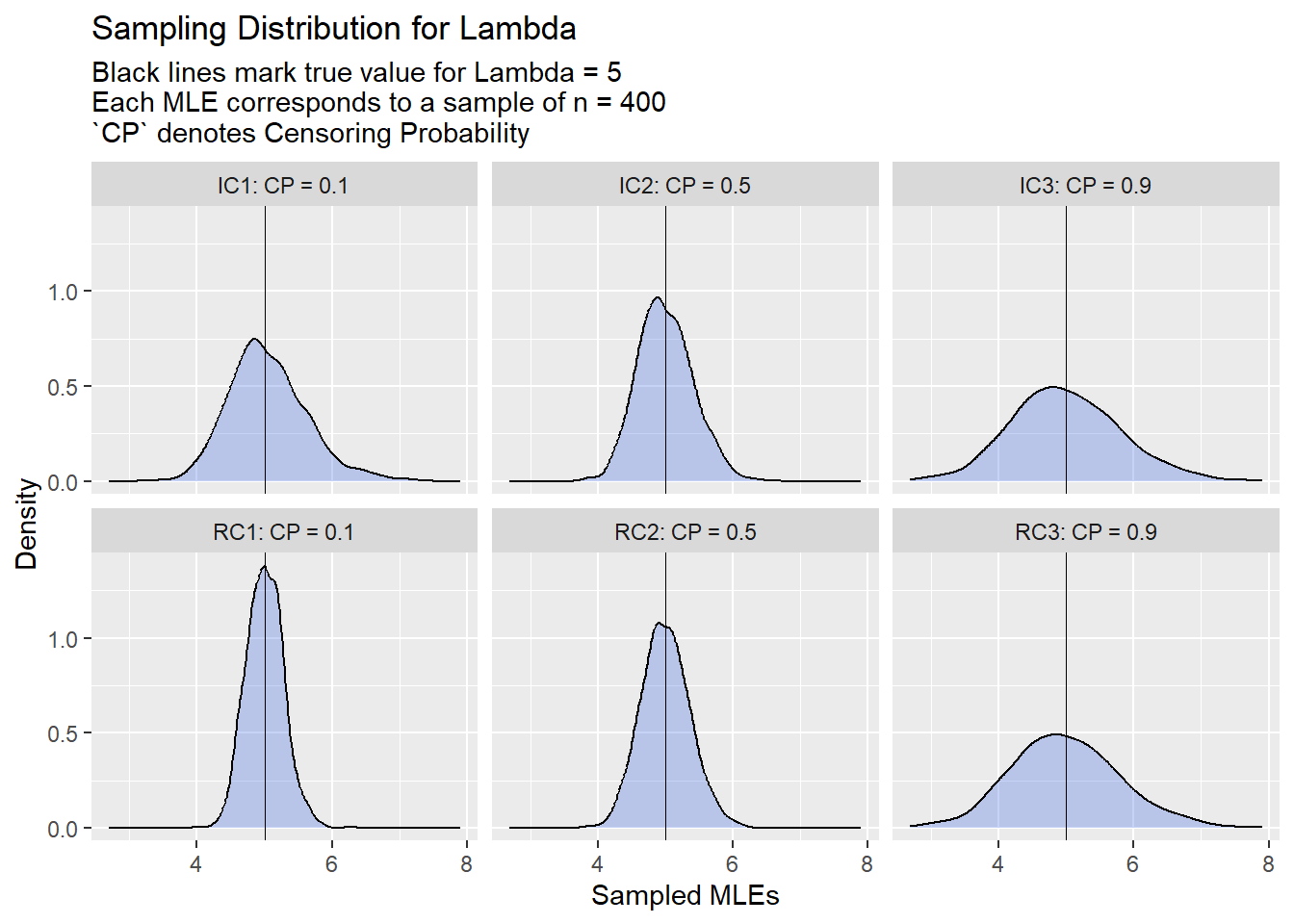
Here we can see how heavier censoring impacts the estimate sampling distributions w.r.t right and current status censoring:
Right Censoring: Clearly heavier censoring hampers the precision of our sampling distribution.
Current Status Censoring: This one is a bit trickier. It would seem that we would want the right censoring and left censoring to occur at approximately equal rates to gain the greatest precision in our sampling distribution, based on the results. Perhaps this mix garners the greatest amount of information.